Goal: Get the robot to travel from one position to another in a known co-ordinate system
To achieve this goal the robot must be able to determine:
- where it is within its co-ordinate system at a given time
- how movement affects its position
Dead Reckoning
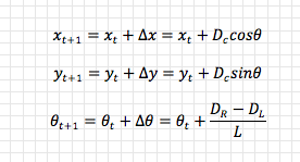
We can solve the first problem using our odometers, trigonometry and some simplifications about what the robot looks like (the wheelbase, L, of our differential drive robot is the distance between its two wheels) and how it moves. Let’s assume that the robot starts at position (xt, yt) and heading θ, then travels distance DC along that heading; the new position (xt+1, yt+1) and heading can be determined as thus:
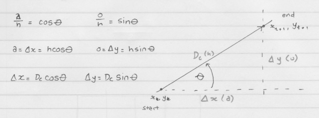
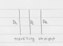
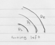
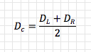
The first challenge is that we don’t actually know DC: the odometers measure the distance travelled by each wheel, DL and DR, which, if the robot is turning, will not be equal. That’s not such a big deal though, because DC must always be between the arcs of each wheel:
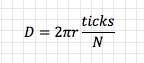
The next challenge is that the odometers don’t actually measure distance in centimeters or meters, they measure distance in ticks (number of state table transitions). Noting that the Pololu rotary encoders being used generate 48 ticks (let N = 48) per revolution of the wheel, that each wheel has a radius, r, and that one full revolution covers a distance equal to the circumference (2πr) of of the wheel (negating any slippage), then the physical distance travelled by a wheel is:
Now we can do this:
x = 0, y = 0, theta = 0
while (true)
{
   ticksLeft = odometer.getTicks(left)
   ticksRight = odometer.getTicks(right)
   distanceLeft = 2 * pi * r * (ticksLeft / N)
   distanceRight = 2 * pi * r * (ticksRight / N)
   distance = (distanceLeft + distanceRight) / 2
   x += distance * cos(heading)
   y += distance * sin(heading)
   heading += (distanceRight - distanceLeft) / L
   sleep(shortTime)
}
This technique is known as dead reckoning: by adding the distance we think we travelled to our previous location we can infer our new location.
It works, but it is error prone. If for any reason the distance we think we have travelled is not actually the distance we have travelled (which can happen for a multitude of reasons, the most common being wheel slippage, where the wheel rotates, but skids: the odometer measures rotation, by the slippage means the wheel does not actually move the same distance over ground).
For the purposes of this experiment, dead reckoning will do: if you’re planning on travelling any real distance, or over uneven terrain, a more accurate positioning system, or ability to reset to known positions, may be required (ie. GPS, known location beacons based on ultrasound, infrared etc).
So far, so good: the robot can now (sort of) determine where it is (assuming a known initial position and heading).
Go to Goal Strategy
The next challenge is to be able to control the robot to go somewhere specific (this is the “go to goal” strategy, ie. “robot, go to x = 10, y = 20!”)
As a starting point, consider the robot as a point-mass, positioned at (x,y), travelling along a straight line with heading θ.
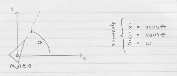
Just as with the dead reckoning, trigonometry can be used to show that its translational (x,y) position will change as a function of its translational velocity, v, (the speed at which it is moving forward along the straight line) and its current heading, θ. This is great news! As a robot all we need to know is our starting position and heading, and then by controlling v and θ we can go anywhere we want.
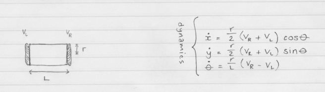
Unfortunately for us, our robot is not a point-mass, nor do we have “direct” control over its translational velocity or heading. We have a left and a right motor and two wheels with a known radius, r, positioned a known distance, L (the wheelbase) apart. The only variables we can control are the velocities (VL and VR) at which the motors spin.
As a programmer, I don’t want to tell my robot “turn your left wheel at 5cm/s and your right wheel at 10cm/s, then adjust left speed to 3cm/s and right to 12cm/s, keep going for 10 seconds and then stop.” Instead, I’d much prefer to say “travel at a heading of 45 degrees at 10cm/s for 10 seconds”, or better yet, “Go to (x = 10, y = 20), there’s a tasty sandwich there I want you to pick up.”
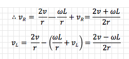
Luckily, by noting that the derivatives in the unicycle model kinematics (our “point mass” model) are the same derivatives as in the differential drive kinematics (our actual model, see also here), that is, they both describe how translational position and heading change with respect to time, we can equate the two models. This allows us to “talk” in terms of translational and angular velocity for the purposes of planning, but then convert them to left and right wheel velocities at the last minute.
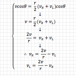
and 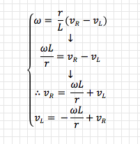
Therefore:

Now, in order to go from point A, to point B, we can say:
- What is my current heading (θ)?
- What heading do I require to get to point B?
- What is the difference between the two headings (Δθ)?
And then, by altering the velocities of the left and right wheels, we can adjust our heading (and translational velocity) such that the difference between the two is reduced and finally our heading matches the required heading.
PID Control
What we now have is a dynamic system (something that changes over time) over which we wish to exert control.
A familiar situation here is cruise control for a car. Driving along toward your summer holiday you get bored of regulating the speed of the car and set cruise control to 100km/h, call this the reference, r. The cruise control system takes a measurement, y, of the current state, x of the variable it is tracking (speed) and compares this with the reference, to create an error (difference), e = r – y.
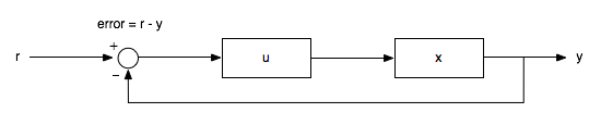
If the cruise control thinks the car is travelling at 90km/h, e = 10km/h and it applies a control signal, u, in this case, acceleration, to try and reduce the error.
If the cruise control thinks the car is travelling at 110km/h, e = -10km/h, and it applies a control signal, u, in this case deceleration, to try and reduce the error.
(As a side note, the reason we distinguish between x and y is because the measurement, based on our sensors, may not actually equal the actual state of the variable. This measurement error represents a known or unknown error introduced by our sensor equipment).
Our robot is much the same, except that we’re not (right now) interested in controlling its speed, we’re interested in controlling its heading, because we know that by adjusting the heading, we can position the robot wherever we like (within reason: we may not be able to make certain turning circles etc). I’ve made a simplification here too: by dropping control of translational velocity and assuming it is constant, we can focus solely on controlling the heading. Control of both variables is beyond the scope of this post.
Just as the control signal for cruise control was the first derivative of the state (acceleration being the first derivative of velocity), the control signal for the robot will be the first derivative of the state we care about: angular velocity (the first derivative of heading/angle). If our error is large (ie. our current heading is really wrong compared to the heading we need to orient ourselves toward point B) then we can apply a large angular velocity (ie. a quick rotation) to ensure we approach our desired heading as quickly as possible.
So, how do we choose the right magnitude of control signal? This is where PID control comes in. PID is an acronym that represents: Proportional, Integral, Derivative.
Let’s go back to the car analogy and say that because we want to get to our reference speed as quickly as possible, we’re going to apply the following rules:
- If e > 0 (ie. we’re below reference speed), u = umax (max acceleration)
- If e < 0 (ie. we’re above reference speed), u = -umax (max braking)
- If e = 0, u = 0 (do nothing)
Now consider what happens if the car is at rest and the reference is 100km/h: the car will accelerate as fast as it can. Similarly, if the car is travelling fast and the reference is set slow, the car will brake as hard as it can. Needless to say, anyone drinking a coffee in the car isn’t going to be happy.
Health and safety aside, you’re quickly going to burn out your actuators, especially when you take real world physics and inertia into account. From standstill, maximum acceleration is going to see the car overshoot the reference velocity, then slam on the brakes, which will undershoot the reference velocity and subsequently rev the accelerator. Because of inertial effects the error will almost always be non-zero, and the actuators will always be working at full action: do that enough and neither will last for long (you’ll probably get car sick too).
Clearly, the control signal should not over-react to small errors: its magnitude must be proportional to the error. If the error is large, our response is also allowed to be large (to hell with onboard coffee drinkers), however if the error is small (ie. we’re only 5km/h off the reference speed), we don’t need to go crazy with the accelerator: just a little bit more will get us there.
If you implement a purely proportional control signal however, you’ll probably notice that while you get close to the reference, you never track it exactly. Small errors accumulate over time that the proportional part of the control signal does not take into account, so we must add an integral part: by integrating the error (with respect to time), we are able to remove more of it.
Whether or not a derivative component is required really depends on the implementation and the physics. It adds fast-rate responsiveness to the control signal (it tracks the derivative of the error over time: if the error is increasing fast, the derivative increases – ie. “quick, this is getting out of control really fast, you need to apply more control!”, if the error is relatively constant, the derivative is a zero component).
Therefore, the control signal (for the robot: angular velocity, or how quickly it is changing its heading) that ends up being applied, consists of P, I and D components:
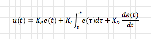
It is our job to pick Kp, Ki and Kd (the PID coefficients) to ensure the control signal, u can make our state, x, approach the reference r (good tracking), without too much oscillation (good stability) as quickly as possible (optimal).
While there are varied methods for selecting Kp, Ki and Kd, often the most realistic (and eventual) solution is simply trial and error: you adjust them until you get the desired result. You can simulate your model and fiddle with them, but when you put the “rubber to the road” (or the robot on the floor), the simulation often drifts away from reality.
Here are some graphs of the simulated results of the robot’s position while travelling from (0,0) to (50,50) using various values of Kp, Ki and Kd:

Kp = 0.01, Ki = 0.01, Kd = 0.00
As can be seen, the heading swings about, never quite reaching its desired reference (θ = π/4 rad) and just when it almost gets there, starts swinging away again. Trying with a more aggressive proportional coefficient:

Kp = 0.75, Ki = 0.05, Kd = 0.00
With these coefficients the control is stable (the heading does not oscillate around its reference) and fairly optimal (the heading reaches the reference quickly). The actual coefficients implemented in the code are different again, taking into account the influence that actual physics of the robot and manner in which the code is implemented have impact.
The Implementation
If you browse through the code you’ll see there is a Controller class, which is responsible for implementing the go to goal strategy by keeping track of the robot’s current position and fulfilling requests to send it to new positions. The implementation sends the robot from a “known” origin of (0,0) at heading 0 rad (ie. pointing out along the positive x-axis) through several waypoints.
The high level implementation is thus:
referenceHeading = getHeading(currentPosition, desiredPosition, currentHeading)

// keep doing this until we get very close to our desiredPosition
while (vectorToTargetMagnitude > sensitivityLimit)
{
   // how long did we sleep since the end of the last iteration (required for PID)
   dt = getActualTimeSlept()

   // get the total distance travelled according to the odometers
   distanceLeft = odometer.getDistance(left)
   distanceRight = odometer.getDistance(right)
   distanceTotal = (distanceLeft + distanceRight) / 2

   // determine how far we've travelled in last iteration
   distanceLeftDelta = lastDistanceLeft - distanceLeft
   distanceRightDelta = lastDistanceRight - distanceRight
   distanceDelta = lastDistanceTotal - distanceTotal

   // determine new position and heading
   currentX += distanceDelta * cos(headingCurrent)
   currentY += distanceDelta * sin(headingCurrent)
   currentHeading += (distanceRightDelta - distanceLeftDelta) / L

   lastDistanceLeft = distanceLeft
   lastDistanceRight = distanceRight
   lastDistanceTotal = distanceTotal

   // how wrong is our current heading required to what we need?
   headingError = referenceHeading - currentHeading

   // determine the required control signal based on the error
   headingErrorDerivative = (headingError - lastHeadingError) / dt
   headingErrorIntegral += (headingError * dt)
   lastHeadingError = headingError

   // control signal is our required angular velocity
   u = (Kp * headingError) + (Ki * headingErrorIntegral) + (Kd * headingErrorDerivative)

   // convert angular velocity to wheel velocities based on kinematic equalities
   velocityLeft = (2*velocityTranslational - u*L) / (2*r)
   velocityRight = (2*velocityTranslational + u*L) / (2*r)

   // convert these velocities to PWM DCs to drive the motors
   motor.setLeftPWM(convertVelocityToPWM(velocityLeft))
   motor.setRightPWM(convertVelocityToPWM(velocityRight))

   // create dt
   usleep(50000)
}
The Real World
Here is a video of the robot running an implementation of the described approach. It has been programmed to move through the following waypoints (which you can see marked out on the floor in black tape if you look closely):
float waypoints[][4] = {
   {45.0, 0.0},
   {90.0, 45.0},
   {0.0, 45.0},
   {1.0, 1.0}
};
Crazily, after all that effort, it still stinks. The tracking to the first waypoint is good, the second not bad, the third a bit flakey but by the fourth we’re way off target. This could be down to odometry errors, unrealistic turning circles, a poor PID implementation or who knows what else. Luckily I’m not building a Mars rover.
Next step: mapping the world with SONAR.


 So far, so good. But how can we put this into practice with the wheel(s) of a robot? A common option is to use a rotary encoder such as the Pololu encoder I have used here. This is an optical encoder and uses two infrared reflectance sensors that shine infrared light onto the inside of the wheel hub, upon which is arranged 12 “teeth” with gaps between them.
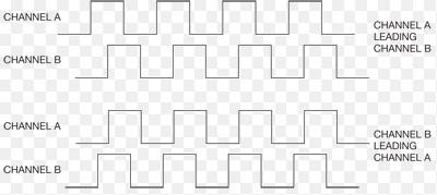
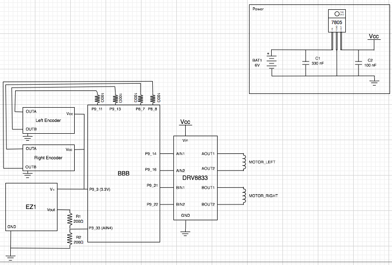
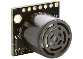 an amplifier and wave generator for them, along with interfacing them back into timers for distance measurement, but a package like the EZ1 takes care of all of this for you.

 supply steady current to the motor (in one of two polarities depending on which control signal is HIGH). This drives the motor at whatever speed it will run for the given input voltage, full speed ahead.
 DC motors are inductive by nature: when current is removed from them their inductance will try to sustain the current and that residual current (called recirculation current) has to have somewhere to flow. When pulse width modulating the H-Bridge inputs, the current is being applied and stopped continually so dealing with the recirculation current is a constant task for the H-Bridge.
