Estimating object location with a single camera and OpenCV

Problem Statement: Determine the physical (real-world) co-ordinates of an object in a scene using a single camera. Concretely, if a reference object (a red cube) is within the field-of-view of oroboto’s camera, determine its position such that oroboto can drive to it. Recall that by dead reckoning, oroboto is aware (more or less) of its own physical co-ordinates within a two-dimensional local frame of reference.

Terminology

In this post the term physical co-ordinates refers to the (x,y) co-ordinates of something in oroboto’s local co-ordinate system / frame of reference. These co-ordinates are specified in units of centimeters and are relative to the location that oroboto was initially powered on, which is considered (0,0) in the physical co-ordinate system.

The term pixel co-ordinates refers to the (x,y) co-ordinates of a given pixel within an image.

Introduction

If we can isolate a reference object within an image we still only possess its pixel co-ordinates: we need a way to convert those to the physical co-ordinates used by the robot.

In this post I’ll discuss using OpenCV to isolate a reference object and then a technique to estimate its physical co-ordinates using only the image from a single camera. A common computer vision (CV) method of determining distance to an object from a camera lens is to use two cameras and the principle of stereoscopic vision to measure depth. While it’s possible to connect multiple cameras to a single Raspberry Pi I wanted to avoid the extra current draw and bulk. I also thought it would be interesting to see the accuracy I could achieve using a simpler approach.

Reference Object, Prerequisites and Assumptions

This technique estimates the physical co-ordinates (x,y) of a reference object (a red cube) of known physical width and height within oroboto’s local frame of reference.

A prerequisite to using the technique is to measure the relationship between the physical dimensions of the cube and how big it appears, in terms of pixels, at various distances from the camera lens. To do this I simply placed the camera at a fixed position and set down a line of markers on the floor at 10cm intervals.

pixel-to-distance

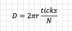
I then took successive images of the cube at each marker and measured how many pixels wide it appeared at each distance. With a table of physical distance (10cm, 20cm, … n cm) and pixel mappings I calculated a regression to get the line of best fit in Excel at arrived at the following pixel-to-distance equation:

pixel-to-distance-eq

If we’re able to isolate the reference object in an image and measure its width in pixels this formula can be used to estimate how far it physically is from the camera lens. This technique makes two major assumptions:

  1. The equation accurately describes the pixel-to-distance relationship across all distancesplane
  2. If you imagine a plane p that runs normal / perpendicular to the ray that extends directly outward from the camera lens and extends through the reference object, that the pixel-to-distance relationship holds true along all points within the camera’s field of view along that plane

Neither of these assumptions are true in all cases which is the primary reason this technique can only estimate position and lacks accuracy.

A final assumption is that the middle of the camera’s field of view aligns exactly with the heading of the robot.

From Pixels to Position

Assume oroboto’s camera has taken an image of the scene and that we’ve used a yet to beopencv1 described technique to isolate the reference cube within the image. We’re now in possession of the (x,y) pixel co-ordinates of the cube as well as its width and height in pixels.

Using the cube’s width in pixels and the pixel-to-distance equation we can estimate (based on assumption #2 above) the physical distance r to the point mid which lies at the intersection of the ray extending directly outward from the camera lens and an imaginary plane p running perpendicular to that ray. Note that mid also lies on the vertical line that equally divides the camera’s image.

opencv-dia1.jpg    opencv2

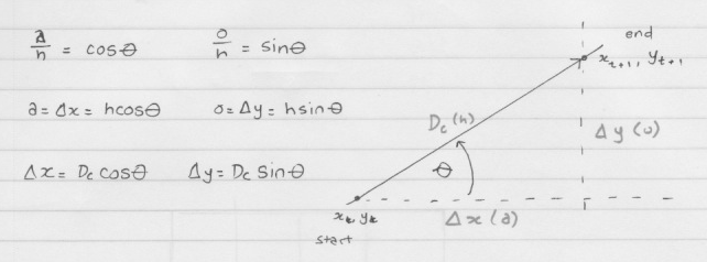
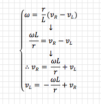
Given that we know oroboto’s physical co-ordinates C and heading q at the time the image was captured, we can use simple trigonometry to estimate the physical (x,y) co-ordinates of mid:

mid-eq.png

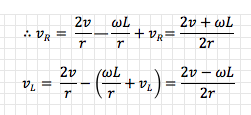
Again based on assumption #2, as the reference cube has known physical width (in centimeters) it is possible to calculate the relationship cmPerPx between pixels and centimeters along plane p (ie. how many cm a pixel represents along that plane). The distance in pixels between mid (recall this lies along the vertical line equally dividing the camera’s image) and the reference cube can then be used to estimate od, the physical distance along plane p between mid (whose physical (x,y) co-ordinates were established above) and the reference cube.

Taking the ray r as the new base of a right-angled triangle (which doesn’t look that right-angled in my diagram) more trigonometry yields q, r and from oroboto’s current position C an estimate of the reference cube’s physical co-ordinates:

obj-eq.png

Isolating the reference cube

The last task is actually locating the red cube within the camera’s image, this is where OpenCV comes in.

In a scene that could contain a multitude of different objects we have two primary “hints” that one of those objects might be ours: its shape and its colour. As we detect and examine objects within the image these will be our primary cues that the object might be the reference cube. Even with these hints we can still be confounded by the fact the shape, which we expect to be a square, could be more trapezoidal or skewed if one of the cube’s faces is off-angle to the camera, and that the colour could appear different depending on lighting conditions. We need to add some robustness to our detection techniques to deal with these cases.

Once the image has been captured it is first converted from RGB (actually BGR, as this is OpenCV’s native representation of RGB) to the HSV (Hue, Saturation, Value) colourspace. Representing the image in HSV is one way to gain some resiliency against varied lighting conditions (shadows, ambient lighting etc).

In HSV, each pixel is specified in terms of its hue (its “core” colour, like “red”), saturation (or “chroma”, this defines the brilliance or intensity of the colour: imagine taking pure red paint and incrementally adding white paint to it such that you move through pinks to pure white) and value (this defines the darkness of a colour or amount of light reflected, imagine taking pure red paint and incrementally adding black paint to it such that you move through rust to pure black). This is useful because it separates colour information from luma (brightness) information. Using HSV, in varied lighting we might expect the saturation and value of the cube’s (red) pixels to vary, but their hue should remain relatively constant. When oroboto is powered on the camera is calibrated to the current environment by placing the red cube in front of it and measuring its average hue. This average, along with a wide range of saturations and values, is used when thresholding incoming images to filter out any pixels that don’t have a similar colour to the cube.

After colourspace conversion, the image is thresholded using OpenCV’s inRange blurred-0function. This takes every pixel of the image and compares it to a range of HSV values measured during calibration, turning potentially red (ie. cube) pixels into white and anything else black. The result is a greyscale image with white pixels wherever red pixels had originally been. This is then smoothed using a Gaussian blur to remove noise (the blur eliminates stray white pixels).

OpenCV offers a range of powerful feature detection algorithms, including findContours, which can extract curves in the image by joining continuous points that have the same colour (which all white pixels in the thresholded image do). We use findContours to extract an external contour (path) around any clusters of white pixels: we hope that one of these clusters resembles a square. For each contour that is found the approxPolyDP function is used to overlay a closed polygon: if that polygon turns out to have 4 sides its aspect ratio is close to 1:1, we’ve found a candidate square. The contours / polygons are iterated to find the best match (the polygon with the aspect ratio closest to 1:1) and if found, this is considered to be the detection of the red cube.

Once isolated the width and height of the cube (in pixels) are known and can be used in the pixel-to-distance equation to start the physical co-ordinate estimation process.

Arduino with Raspberry Pi I2C Slave

I²C (“Inter-integrated circuit”, which as a trademark of Phillips is more generically implemented by other vendors as “Two Wire Interface” or TWI) is a synchronous serial interface that is often used to connect peripheral devices (think EEPROMs, gyroscopes, accelerometers, wheel encoders etc) to microcontrollers. Electrically, it requires only two “wires” between each device, a clock line (SCL) and a data line (SDA) and these lines can be shared as a common bus between multiple devices, allowing for a multi-master and multi-slave environment. Each slave on the bus has a unique address within a 7-bit address space.

Both the ATmega32U4 (the microcontroller included on the Romi 32U4 control board) and the Raspberry Pi (as functionality included in its Broadcom BCM2835 (or later) SOC), include hardware allowing them to function as either I²C master or slave. This presents an opportunity to allow simple communication between the two. But why would this be useful and how should we choose who gets to be master and who is a slave?

As an 8-bit microcontroller with 32kbyte program memory the ATmega32U4 is clearly limited in its capabilities. There is no room or compute power for more advanced functionality, such as computer vision, that we want oroboto to be capable of. However, if we couple it with a more powerful system, such as the Raspberry Pi, a whole new set of opportunities open up: CV, communication over WiFi, co-operative robotics. The Romi 32U4 control board that the newer iterations of oroboto are using has a female 40-pin header with pinout and mounting holes that are compatible with the Raspberry Pi HAT (Hardware Attached on Top) specification. It directly connects the ATmega32U4’s SDA and SCL lines to those of the Raspberry Pi (which actually has multiple I²C buses) and also routes power from the Romi’s 6x AA batteries to the Pi. You simply have to slot the Pi onto the top of the control board and you now have a powerful robotics platform: the ATmega32U4 can take care of low level functionality like motor control and anything that is timing sensitive, such as reading wheel encoders, and higher level logic, such as navigation strategy and communication can be offloaded to the Pi. Even when adding extra hardware, such as the Raspberry Pi camera, I can power the whole lot for around 45 minutes on the 6x AA batteries.

Having the Raspberry Pi powered up and running alone obviously isn’t sufficient for an integrated system: it needs to be able to communicate with the Arduino via I²C.  However, getting this working can have its complications. There is a known bug in Broadcom Serial Controller (BSC) of the Broadcom BCM2835 SOC (the chip that contains the Raspberry Pi’s CPU, RAM, video and other peripherals such as I²C) that corrupts data when I²C slaves (such as the Arduino) implement a technique known as clock stretching to slow down communication on the bus. It would seem that the hardware TWI (I²C) module in AVR microcontrollers does stretch the clock when the AVR is a slave and this has and is causing trouble for people trying to connect it to a Raspberry Pi because of the Broadcom bug. I should note that I haven’t been able to directly verify whether the Broadcom issue exists in later versions of the BCM283x as used in Raspberry Pi 2 and 3 models.

To work around these issues, the Romi team have created an alternative to the standard Arduino Wire.h I²C library: the PololuRPISlave library which configures the Arduino as an I²C slave and adds timing hacks at the right places to allow successfully communication with a Raspberry Pi master at relatively high speeds. Phew, saved! But… no, oroboto of course has to be more complicated than that.

As previously mentioned, the Romi control board includes the LSM6DS33 IMU (which we need for a gyroscope) and for a while I was also experimenting with a 3-axis magnetometer, the QMC5883L: the readings from both of these units require the Arduino to operate as an I²C master and the sensors as I²C slaves. The pre-canned libraries (which I wasn’t inclined to reimplement) for the LSM6DS33 and QMC5883L configure the Arduino as an I²C master and PololuRPISlave configures it as a slave. Using them together doesn’t work out of the box. While it does seem to be possible to run the Arduino as a mixed master / slave it was a level of fiddling and patching existing libraries I wanted to avoid if possible. The solution I arrived at was counter intuitive from the perspective of “big is master, little is slave” but works: the Arduino remains the single master on the I²C bus and I configure the Raspberry Pi as an I²C slave (even though in the long run it’s the “command module” of the overall integrated system).

The pigpio package (and its Python bindings) expose the bsc_i2c() function that allow the Pi to operate as an I²C slave. After installing pigpio on the Raspberry Pi (it starts a daemon that implements the functionality exposed by its bindings) it’s simple to configure a slave address for the Pi and register for an interrupt when a master attempts to communicate with that address:

import pigpio

pi = None
slave_addr = 0x13

def i2cInterrupt():
   global pi
   global slave_addr
   status, bytes_read, data = pi.bsc_i2c(slave_addr) 

   if bytes_read:
      doYourThing(data)

pi = pigpio.pi()
int_handler = pi.event_callback(pigpio.EVENT_BSC, i2cInterrupt)
pi.bsc_i2c(slave_addr)

Later posts will go into more detail, but the code that runs on oroboto’s Raspberry Pi essentially:

  1. Sets up a UDP server listening for data from botLab (the companion macOS application to send commands and receive telemetry from oroboto)
  2. Sets up the Raspberry Pi as an I²C slave
  3. Is periodically polled by the Arduino (acting as I²C master) to see whether any new commands have arrived from botLab (ie. “navigate to waypoint x,y”)
  4. If a command has been received, sends the command payload back to the Arduino for execution


Measuring rotation with the LSM6DS33 Inertial Measurement Unit

oroboto-with-centroid
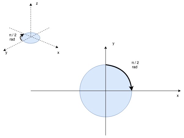
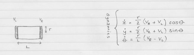
A differential drive robot’s two wheels are placed horizontally adjacent to each other, as if connected by an axle (their “axis”), and their speed is independently controllable. On most (all?) differential drive robots the axis running through the two wheels also runs through the centre of the bot so that any rotation occurs through its centroid in the x-y plane.

As mentioned in the previous post, there are times, such as when a significant correction in heading is required, when we want the robot to “spin on a dime”: that is, rotate around its centroid without changing its (x,y) position. This can be achieved using odometry. In order to rotate π / 2 rad (90 deg) each wheel must travel a distance of arclen, which is defined by the wheelbase (distance between the wheels) of the robot and the desired rotation angle. So, one implementation of rotation can simply be to rotate both wheels in opposite directions at the same speed and periodically (often) check their odometry readings: once they’ve travelled arclen the robot has rotated the required angle.

odometry

The problem with this approach is as mentioned in the previous post: the voltage/speed response curves of each motor are not identical. The Romi’s motor libraries accept a signed signed 16-bit integer (capped to -300 to +300) as input, which is converted into a PWM signal to the DRV8838 motor driver, which ultimately is represented as a control voltage to the motor. Instructing both motors to spin at “+100” will result in slightly different actual speeds in each motor. The net result is slip on one wheel (and/or drag on the other) and an invalidation of the assumption that because you’ve measured a distance travelled of d (via odometry) for one wheel that the arclen travelled was really d. In other words, you under or over rotate. While this seems theoretical, in practice it quickly manifests itself. Box test failed.

Luckily, the Romi’s control board has a built-in LSM6DS33 inertial measurement unit. This consists of 3-axis accelerometer and 3-axis gyroscope. Gyroscopes measure rotational motion (angular velocity), that is, how fast they (or the fixed body they’re attached to, in this case, oroboto) are rotating around a given axis. This angular velocity is measured in degrees per second. Just as we can measure (x,y) displacement by integrating translational velocity over time, we can measure angular displacement (rotation) by integrating angular velocity over time.

gyro

The course correction mode previously implemented with odometry becomes simpler:

  • At t = 0 assume angle_rotated = 0
  • Set speed of both motors to s
  • Periodically measure (sample) angular velocity around the z-axis (the axis that runs through the center of the robot, “pinning” it to the floor: this corresponds to its change in heading (the interval of this periodic check is dt)
  • Integrate the angular velocity with respect to dt, yielding angle_rotated (degrees rotated since t = 0)
  • Stop when angle_rotated >= desired rotation

This is a simplification; in the code you can see the LSM6DS33 actually reports angular rotation in “gyrodigits” (digits per second, or DPS), which allow the device to support multiple levels of sensitivity / granularity and that it’s necessary to calibrate the gyroscope before use. Calibration allows some of the random noise the gyroscope experiences to be removed from each sample.

Each sample of the gyroscope’s angular velocity around an axis contains a random amount of noise (ie. some samples will under-report angular velocity, others will over-report angular velocity): continued integration of these samples accumulate that noise and result in drift: the integrated value (ie. the amount of rotation that has occurred since we started measuring) will become less accurate over time. Calibration helps to remove some of this noise but cannot account for all of it. If using the gyroscope to measure rotation over a long time period, this is a problem. Thankfully, course correction routines, where the robot is trying to correct for a specific amount of heading error, are short-lived and essentially “reset the drift clock” each time they start. At the start of the routine, we are seeking to correct for err degrees heading error from the current heading, which for the purposes of the correction, is considered “0 degrees”. The integration of angular velocity only has to occur until err degrees of rotation has occurred from that initial 0 degree starting point. Because this rotation occurs quickly (the robot can spin 360 degrees in under a few seconds, even when moving slowly) there isn’t time for drift to accumulate and as such the gyroscope is accurate under these conditions as illustrated in the videos below.


Drift becomes a problem when trying to use the gyroscope to measure rotational change over a longer time period. Consider a pilot who takes off along a runway with known heading (ie. perhaps it runs due north-south) and who has reset his gyroscope to “0 degrees” when facing north up the runway before takeoff. At this time, the gyroscope reading is accurate. After takeoff, his gyroscope is continually integrating angular velocity (in whichever axes it cares about, hopefully all three) with respect to that initial reset on the runway. Over time, a few hours into his trip, the gyroscope will have accumulated significant error through drift and will no longer be identifying accurate headings. A similar situation occurs with oroboto when using the gyroscope as an alternative to odometry when measuring change in heading between PID loop iterations. In this case the robot continues integrating gyroscope readings as it transits between waypoints, each time adding or subtracting from its last known heading. Over time, gyroscope drift causes these measurements to become less and less accurate and leading to incorrect heading adjustments for the PID loop. Box test failed.

As a method based on integration, odometry suffers exactly the same drift problems as the gyroscope, but in my testing, under the distances travelled (less than 100 meters), odometry was providing better accuracy than the gyroscope method.

One way to correct for drift is to combine the readings of a drift prone sensor (such as a gyroscope or wheel odometry) with the readings of a non-drift prone sensor, such as a magnetometer. This is called sensor fusion, a topic that deserves way more than one post alone.

Before delving into that rabbit hole, however, my next post will focus on interfacing the Romi to a Raspberry Pi I2C slave. This gives oroboto a huge amount of computing power to execute higher level navigational tasks and allows for simple robot-to-robot and robot-to-controller communication over WiFi.

oroboto v2.0

It’s been a long time between posts but I’ve not been idle. I recently discovered the Romi differential-drive chassis from Pololu and have been experimenting with two robots I’ve built on top of it. Unlike the initial iterations of oroboto, which involved a lot of sticky tape and solder bridges to bring everything together on top of the Beaglebone Black (BBB), Romi is a set of neatly interchangeable components including the chassis (with in-built 6xAA battery compartment), 2x 120:1 DC motors, ball caster and wheels. Pololu sell a control board that sits neatly on top of the chassis and provides an ATmega32U4 AVR (Arduino-compatible) microcontroller, DRV8838 H-bridge motor drivers, power distribution circuit and an LSM6DS33 3-axis accelerometer and gyroscope. The motors are easily interfaced with magnetic Hall-effect quadrature encoders to enable odometry and the control board has a header for direct interfacing with a Raspberry Pi. In short, it provides everything the original oroboto had (albeit with a Raspberry Pi rather than a Beaglebone Black) but in a more robust package with less assembly required.

orobotos

Porting the original oroboto code to the Romi was trivial: all of the interface code that poked the BBB’s GPIOs and interrupts got chucked out and replaced with Arduino-specific library calls but the core PID loop and navigation logic remained. Earlier readers may recall the significant problems I had getting oroboto to “hit its waypoints” while executing a transit. I had hoped the port to Romi would result in immediate performance improvements for two reasons: a) the Romi’s motors were more highly geared (120:1 vs 100:1) which should grant slightly higher rotary encoder resolution, but more importantly; b) everything was running directly on the AVR instead of jumping back and forth between the kernel and user-space on the BBB, which should have resulted in much finer timing and accuracy. The original BBB code relied on a select() on a file descriptor for the user-mode process to learn of GPIO interrupts from the rotary encoder and on a fairly opaque PWM implementation to drive the motors. By the time the feedback loop from input to output was complete there was a lot of context switching and I couldn’t guarantee how the kernel would schedule the oroboto control process. In contrast, on the AVR, everything is running in a single “thread” and timing control is deterministically related only to the running code.

Needless to say, I was disappointed. Well, I wasn’t totally disappointed, it’s always nice after porting a project from one platform to another that it runs at all, but for my “box test” (getting oroboto to transit between 4 waypoints that define the corners of a 1m x 1m square) the accuracy was still fairly miserable. I ruminated on the problem for a few days and realised the obvious: you can’t make pigs fly.

Without giving it due consideration, I think I’d been hoping the PID implementation would magically cause oroboto to spin on a dime once it reached one waypoint and began the transit to the next, but in reality the magnitude of control signal change is often too high to map onto the physical constraints of the motor. Even if it was mappable, such a sudden change in torque can cause slip and inaccurate odometry readings. To be specific, the DC motor speed is varied by controlling its input voltage: this is achieved via a PWM signal sent to the DRV8838 motor driver. Assume the motor’s input voltage range is 0V to 5V and this maps to a (fictitious, I haven’t actually measured min and max RPM)  speed range (post gearing) of 0RPM to 50RPM (discounting for the fact the mapping is not linear, which is a further complication). At any iteration, the PID loop is trying to correct for the heading error (the error between the robot’s current heading and the heading it needs to travel on to reach its target waypoint) by adjusting the speed (RPM) of the left and right motors to create the required amount of “turn” to the left or right. If the robot has reached a waypoint and its next waypoint requires a 90 degree turn to the left (ie. to the adjacent corner of the “box”), the heading error is 90 degrees, which translates into a large positive control signal to right motor (“turn forwards at 200 RPM!”) and a large negative control signal to the left (“turn backwards at 200RPM!”). The main problems in this scenario are that the magnitude of the control signal (as measured in RPM) can exceed the physical capabilities of the motor and that the response curve of each motor (the mapping between input voltage and output RPM) is neither linear nor matched to that of the other motor. While you might hope these differences “come out in the wash”, that wasn’t my experience. The first problem is somewhat akin to the turning circle of a car: you simply can’t turn at an angle greater than that allowed by the physics of the steering mechanism.

I decided to simplify the problem and let the differential-drive robot do what it does best: spin. At each iteration of the PID loop, if the heading error exceeds 30 degrees, I break into a “course correction” mode that stops forward transit and (relatively) slowly spins the motors in opposite directions to achieve the amount of “on a dime” turn required to correct the heading error. Once corrected, I let the PID loop take over “straight line” correction again. This made a significant improvement in accuracy during the box test and even allowed the robot to complete several transits of more complicated box patterns with little displacement error. However, the problem of mismatched response curves between motors remained. During this course correction mode, the arc length that must be travelled by one of the motors to achieve the rotation required to correct for the heading error is computed and then the odometry of that wheel is monitored until the arc length has been traversed: in other words, it assumes that if that wheel has travelled a certain distance then the other wheel has travelled exactly the same distance in the opposite direction and thus that the required rotation has occurred. This is a poor assumption: the motors do not have the same response curves and when instructed to spin at the same speed, a margin of error (which differs based on the requested speed due to non-linearities in the motors themselves) is introduced. The net result is that over or under rotation occurs.

While I did spend some time writing motor calibration code to do simple lookup table based left-to-right response curve correction I settled on a different approach: ditch odometry for the rotation measurement and use the onboard gyroscope instead.

The next few posts will discuss using the LSM6DS33 inertial measurement unit (IMU) gyroscope; why sensor fusion between an accelerometer and gyroscope can’t ever give better measurements of yaw; how to interface the AVR to a Raspberry Pi acting as an I2C slave (and why you might want to do that); introducing peer-to-peer communication over WiFi between two robots for co-operative navigation and using AWS Rekognition and OpenCV to give oroboto eyes.

3D Network Visualisation

The lack of robot related posting is due to a minor course deviation into a work-related minefield. Mine sweepers have been deployed and we expect to be back on our original trajectory momentarily. The crew wish to thank you for your patience.

In the interim, I have been writing Interconnect, a 3D network connectivity visualisation tool for Mac OSX and CampSight, an iOS application to locate nearby campsites in Australia and the United States even when Internet connectivity is unavailable.

The next stage for oroboto will be improved ultrasonic ranging capabilities before moving onto navigation with SONAR-derived local area maps.

BeagleBone Black Wifi

While tuning the PID loop and debugging the ultrasonic range finding code (more on that to come) in oroboto I’ve been writing log files to its flash for subsequent analysis using dotVision.

A log line contains the following data:

timestamp x y logtype waypoint

token data type description
timestamp
float time in seconds since the first log entry (intrinsically 0.0)
x
float x co-ordinate
y
float y-coordinate
logtype
string class of entry (for dotVision colour markup etc)
waypoint
int whether or not this is a waypoint marker

There were two reasons for recording this data:

  1. Keep track of where the robot thought it was (x,y co-ordinates) at a given time (to allow for comparison to where it really was)
  2. For ultrasonic range finding, keep track of where the robot detected obstacles (to allow for comparison to where they actually are)

While the timestamps are useful, because they allow dotVision to play the log back “in realtime” I still had to try and remember where the robot was at that time in order to make any meaningful comparisons for #1. This turned out to be a fruitless effort.

Better solution: pipe the data back to dotVision in realtime over a wireless connection.

dotVision (updated on git) has now been updated with a UDP server (uses Grand Central Dispatch to put a dispatch source around the socket and then schedules “dot” additions into the dotLog on the main UI thread for drawing) and the DotLog class on the BBB has a mini UDP client in it.

Which brings up the next question: what’s the ideal physical layer to send this over? The two obvious choices are 802.11(whatever) or BlueTooth. I had a spare D-Link DWA-131 revB USB wifi adapter lying around so I gave that a shot…

DWA-131 revB Power Requirements

First things first, you’re gonna need more power. I had limited success getting the DWA-131 revB running when tethered via USB and no success at all when running off the measly 5x AA cell power supply I had jury rigged. Scratch that, time for a LiPo.

Lithium-based battery chemistry has come a long way and as any RC fan can attest, LiPo (lithium polymer) batteries can deliver a significant amount of current in a small form factor (just be careful charging them, they also make great fireworks).

zippy2s

I picked up a few Zippy 2200mAh 2S batteries (2S meaning 2 cells in series, so 7.4V at full charge) and rejigged the robot chassis a bit to house one of them (and we now have an on/off switch, what progress!). This keeps the BBB, wifi adapter and motors happy for at least an hour in the testing I’ve been doing.

“Look ma, no hands!”

Now for the meaty bit. Once this is done the robot can boot the default BBB Angstrom Linux distro and be immediately accessible directly via WiFi. This assumes you’re connecting to an infrastructure mode network using WPA2.

  • Download the firmware for the WiFi chipset used by the DWA-131 (an RTL8192CU) from here and copy it into /lib/firmware/rtlwifi
  • Load the kernel module at boot:
# echo rtl8192cu > /etc/modules-load.d/rtl8192cu.conf
# update-modules
  • Disable connman, it’s a con, man:
# systemctl disable connman.service
  • Define the properties for your wireless network and the NIC you’ll be using (wlan0). Note that unlike as mentioned in the references, there is no pre-up command here. This happens in /etc/network/interfaces:
auto wlan0
iface wlan0 inet static
   address X.X.X.X
   netmask mask.mask.mask.mask
   gateway your.gateway.ip
   wireless_mode managed 
   wireless_essid "YOUR_ESSID"
   wpa-driver nl80211
   wpa-conf /etc/wpa_supplicant.conf
   post-down killall -q wpa_supplicant
  • Generate the hash for your WPA pre-shared key using wpa_passphrase, follow the prompts and then look for the psk line, you’ll be wanting to put that in your wpa_supplicant configuration file, /etc/wpa_supplicant.conf:
fast_reauth=0
ap_scan=1
network={
 scan_ssid=1
 proto=WPA2
 key_mgmt=WPA-PSK
 pairwise=TKIP
 group=TKIP
 ssid="YOUR_ESSID"
 psk=long_hex_string_from_wpa_password

}

  • We now need to ensure the DWA-131 firmware is loaded at boot time by configuring the kernel module with the USB device ID of the adapter. Angstrom is using systemd for boot time initialisation scripts so I just wrote a little service that runs when the networking stack comes up. The key here is to ensure it runs before we try to bring the interface up (see wifi.service below), note the Before condition.  The contents below goes into /lib/systemd/system/wifidriver.service:
[Unit]
Description=wifidriver
Wants=network.target
Before=wifi.service
[Service]
Type=oneshot
RemainAfterExit=yes
ExecStart=/home/root/wifidriver.sh
[Install]
WantedBy=multi-user.target
  • The /home/root/wifidriver.sh it references is simple:
#!/bin/sh
echo "2001 330D" | tee /sys/bus/usb/drivers/rtl8192cu/new_id
  • Enable the service so it runs at boot:
# systemctl enable wifidriver.service
  • The last step is to get the interface itself to come up (as we disabled connman which technically was meant to do it on demand, but seems to be rather average at that job). This is again done with a simple systemd service. The contents below goes into /lib/systemd/system/wifi.service:
[Unit]
Description=wifi
Wants=network.target
Before=network.target
BindsTo=sys-subsystem-net-devices-wlan0.device
After=sys-subsystem-net-devices-wlan0.device

[Service]
Type=oneshot
RemainAfterExit=yes
ExecStart=/home/root/wifi.sh
ExecStop=/bin/sh -c "ifdown wlan0"

[Install]
WantedBy=multi-user.target
  • The /home/root/wifi.sh it references (the sleep is just to give the driver time to load the firmware and boot the device):
#!/bin/sh
sleep 10
ifup wlan0
  • Finally, enable the service so it runs at boot:
# systemctl enable wifi.service


The act of bringing up the interface should cause wpa_supplicant to run and authenticate against your network (it will remain running as a daemon to handle rekeying etc).

Reboot and hopefully you’ll be able to SSH in directly without the USB tether.

References:

  1. Ubuntu 12.04 – Install D-Link DWA-131 rev. B1 wifi adapter
  2. Auto connect to a wireless network (Ångström Linux)

Next research project: low power BlueTooth instead of WiFi. But before then, some notes on ultrasonic range finding.

Go To Goal Strategy Implementation

If you take a look on GitHub there is now an example implementation of the Go to Goal strategy described in the previous post.

  • The bulk of the logic is in the file modules/controller.cpp
  • Additional support libraries have been added, such as:
    • gpio: wrapper to configure BBB GPIOs (used by the odometer)
    • odo: a basic odometry implementation to measure distance travelled by a wheel using optical encoders
    • led: wrapper to configure and interface with the onboard user LEDs
    • logger: simple text-based logging abstraction
    • dotlog: class that can create files to be read by dotVision

I’ve also committed the dotVision project, a simple Objective C application (provided as an X-Code project) for OSX that takes log files of data from the robot and plots it either on the same timescale as the data was created or in one hit. This is a useful debugging tool to quickly visualise 2D data that the robot is / was processing (future improvements will include socket support to take a feed of data in realtime (ie. via WiFi) to plot progress).

dotVision

The screenshot shows the dead reckoned position co-ordinates of the Go to Goal strategy module (ie. where it thought it was in its 2D co-ordinate system as it followed the defined waypoints). It would of course be interesting to be able to overlay this with the actual measured position of the robot.

The trace is black while the strategy thinks it is still far from the next waypoint, red as it believes it is approaching the waypoint and yellow when it stops as close as it can to the waypoint.

You can see that while it hits the first and second waypoints easily, the interaction between the PID controller tuning and the simplistic implementation of “set forward velocity” leads to a very loose turning circle as it adjusts its heading for the third waypoint.

Implementation Challenges

There were quite a few issues encountered (and not fully resolved) while implementing the current Go to Goal strategy including:

Knowing when to stop

When the strategy sets out for a waypoint it takes its current (believed) position (in theory the middle point of the robot between the wheels) and heading and works out the new heading required for the robot to be “facing” (directed toward) the next waypoint. It then drives at a set forward velocity until its (believed) heading is as close as possible to the required heading (the “set forward velocity” is modulated by changes to the left and right wheel velocities required to make any turns needed to track the reference heading: this is the job of the PID loop whose reference variable is simply the heading).

(As a side note this simplistic implementation means that it’s difficult/impossible for the strategy to deal with waypoints that are too close together.)

Consider the very real possibility that due to a combination of PID tuning and physics the robot simply isn’t tracking well to its required path: perhaps it’s at (90,45) and wants to move to (0,45) but never quite manages to hit the straight line between them: at some point it will go past the target waypoint and … probably keep driving off into the distance.

The simple solution implemented in the current strategy is to measure a vector between the current position and the waypoint.

If the vector is noted to be “small enough” (relative to the size of the robot) the strategy believes it has reached the waypoint and stops.

If the vector does not ever get “small enough” the strategy waits until it sees the size of the vector increasing (on the logic that for the bulk of the transit, other than some initial turning, from waypoint A to waypoint B, the vector should shrink) and when it notes a prolonged increase (ie. we keep getting further and further from the target) that is significant in the context of the initial vector between the two waypoints it “gives up” and assumes any further transit is only going to place it further from its goal.

Determining how often to reset the reference heading between waypoints

Initially the strategy calculated the reference heading just once (as described above) at the time it began a transit from one waypoint to another.

The initial reasoning behind this was that the error from dead reckoning was assumed to be large (ie. once the journey from A to B had started the “believed” position was likely to be increasingly wrong). As such, recalculating the reference based on that dodgy position was just going to cause issues (this is somewhat of a moot point though: if the incremental believed position is wrong, the “final” believed position (ie. where we think we are vs where we actually are when we arrive at the target waypoint) will also be wrong and hence the next reference heading calculation for the subsequent waypoint will also be wrong.

In reality the dead reckoned position over the distances of the experiment (less than 1m x 1m so not really useful or significant) was fairly accurate, so continuously recalibrating the “new” reference heading during the transit, based on “believed” position, rather than just once per transit, seemed to give better outcomes than doing it just once.

Achieving a reasonable balance between PID loop tracking, algorithm and physical limitations

As can be seen in the dotVision plot, the strategy of using a continuous forward velocity causes some issues when large turning circles are required.

The robot itself is capable of turning on a pin: a better strategy could take advantage of the physical characteristics of independent wheel rotation to:

  • use smaller forward velocities when enacting large heading corrections to minimise lateral / translational drift
  • adopt a separate “turn on a dime” strategy when starting out from a given waypoint

Next Steps

Rather than continuing to explore some of the adaptions above to the strategy itself the next steps for this robot will be to use the ultrasonic transducer to begin taking measurements as it moves and build a map of the surroundings.

In future this information can then be used by the “Go to Goal” strategy to avoid obstacles, ideally I’d like to see the robot adapt a new path when an obstacle appears in between two of its desired waypoints.

Beaglebone Black PID Control and Go to Goal

Goal: Get the robot to travel from one position to another in a known co-ordinate system

To achieve this goal the robot must be able to determine:

  • where it is within its co-ordinate system at a given time
  • how movement affects its position

Dead Reckoning

We can solve the first problem using our odometers, trigonometry and some simplifications about what the robot looks like (the wheelbase, L, of our differential drive robot is the distance between its two wheels) and how it moves. Let’s assume that the robot starts at position (xt, yt) and heading θ, then travels distance DC along that heading; the new position (xt+1, yt+1) and heading can be determined as thus:

Screen Shot 2014-10-26 at 10.39.03 AM

Screen Shot 2014-10-26 at 10.37.55 AM

The first challenge is that we don’t actually know DC: the odometers measure the distance travelled by each wheel, DL and DR, which, if the robot is turning, will not be equal. That’s not such a big deal though, because DC must always be between the arcs of each wheel:

Screen Shot 2014-10-26 at 10.33.53 AMScreen Shot 2014-10-26 at 10.33.49 AMScreen Shot 2014-10-26 at 10.34.55 AM

The next challenge is that the odometers don’t actually measure distance in centimeters or meters, they measure distance in ticks (number of state table transitions). Noting that the Pololu rotary encoders being used generate 48 ticks (let N = 48) per revolution of the wheel, that each wheel has a radius, r, and that one full revolution covers a distance equal to the circumference (2πr) of of the wheel (negating any slippage), then the physical distance travelled by a wheel is:

Screen Shot 2014-10-26 at 10.38.37 AM

Now we can do this:

x = 0, y = 0, theta = 0
while (true)
{
   ticksLeft = odometer.getTicks(left)
   ticksRight = odometer.getTicks(right)
   distanceLeft = 2 * pi * r * (ticksLeft / N)
   distanceRight = 2 * pi * r * (ticksRight / N)
   distance = (distanceLeft + distanceRight) / 2
   x += distance * cos(heading)
   y += distance * sin(heading)
   heading += (distanceRight - distanceLeft) / L
   sleep(shortTime)
}

This technique is known as dead reckoning: by adding the distance we think we travelled to our previous location we can infer our new location.

It works, but it is error prone. If for any reason the distance we think we have travelled is not actually the distance we have travelled (which can happen for a multitude of reasons, the most common being wheel slippage, where the wheel rotates, but skids: the odometer measures rotation, by the slippage means the wheel does not actually move the same distance over ground).

For the purposes of this experiment, dead reckoning will do: if you’re planning on travelling any real distance, or over uneven terrain, a more accurate positioning system, or ability to reset to known positions, may be required (ie. GPS, known location beacons based on ultrasound, infrared etc).

So far, so good: the robot can now (sort of) determine where it is (assuming a known initial position and heading).

Go to Goal Strategy

The next challenge is to be able to control the robot to go somewhere specific (this is the “go to goal” strategy, ie. “robot, go to x = 10, y = 20!”)

As a starting point, consider the robot as a point-mass, positioned at (x,y), travelling along a straight line with heading θ.

Screen Shot 2014-10-26 at 11.04.41 AM

Just as with the dead reckoning, trigonometry can be used to show that its translational (x,y) position will change as a function of its translational velocity, v, (the speed at which it is moving forward along the straight line) and its current heading, θ. This is great news! As a robot all we need to know is our starting position and heading, and then by controlling v and θ we can go anywhere we want.

Unfortunately for us, our robot is not a point-mass, nor do we have “direct” control over its translational velocity or heading. We have a left and a right motor and two wheels with a known radius, r, positioned a known distance, L (the wheelbase) apart. The only variables we can control are the velocities (VL and VR) at which the motors spin.

Screen Shot 2014-10-26 at 11.05.52 AM

As a programmer, I don’t want to tell my robot “turn your left wheel at 5cm/s and your right wheel at 10cm/s, then adjust left speed to 3cm/s and right to 12cm/s, keep going for 10 seconds and then stop.” Instead, I’d much prefer to say “travel at a heading of 45 degrees at 10cm/s for 10 seconds”, or better yet, “Go to (x = 10, y = 20), there’s a tasty sandwich there I want you to pick up.”

Luckily, by noting that the derivatives in the unicycle model kinematics (our “point mass” model) are the same derivatives as in the differential drive kinematics (our actual model, see also here), that is, they both describe how translational position and heading change with respect to time, we can equate the two models. This allows us to “talk” in terms of translational and angular velocity for the purposes of planning, but then convert them to left and right wheel velocities at the last minute.

Screen Shot 2014-10-26 at 10.21.12 AM

and Screen Shot 2014-10-26 at 10.29.56 AM

Therefore:

Screen Shot 2014-10-26 at 10.32.46 AM

Screen Shot 2014-10-26 at 10.39.27 AM

Now, in order to go from point A, to point B, we can say:

  • What is my current heading (θ)?
  • What heading do I require to get to point B?
  • What is the difference between the two headings (Δθ)?

And then, by altering the velocities of the left and right wheels, we can adjust our heading (and translational velocity) such that the difference between the two is reduced and finally our heading matches the required heading.

PID Control

What we now have is a dynamic system (something that changes over time) over which we wish to exert control.

A familiar situation here is cruise control for a car. Driving along toward your summer holiday you get bored of regulating the speed of the car and set cruise control to 100km/h, call this the reference, r. The cruise control system takes a measurement, y, of the current state, x of the variable it is tracking (speed) and compares this with the reference, to create an error (difference), e = r – y.

Screen Shot 2014-10-26 at 11.20.56 AM

If the cruise control thinks the car is travelling at 90km/h, e = 10km/h and it applies a control signal, u, in this case, acceleration, to try and reduce the error.

If the cruise control thinks the car is travelling at 110km/h, e = -10km/h, and it applies a control signal, u, in this case deceleration, to try and reduce the error.

(As a side note, the reason we distinguish between x and y is because the measurement, based on our sensors, may not actually equal the actual state of the variable. This measurement error represents a known or unknown error introduced by our sensor equipment).

Our robot is much the same, except that we’re not (right now) interested in controlling its speed, we’re interested in controlling its heading, because we know that by adjusting the heading, we can position the robot wherever we like (within reason: we may not be able to make certain turning circles etc). I’ve made a simplification here too: by dropping control of translational velocity and assuming it is constant, we can focus solely on controlling the heading. Control of both variables is beyond the scope of this post.

Just as the control signal for cruise control was the first derivative of the state (acceleration being the first derivative of velocity), the control signal for the robot will be the first derivative of the state we care about: angular velocity (the first derivative of heading/angle). If our error is large (ie. our current heading is really wrong compared to the heading we need to orient ourselves toward point B) then we can apply a large angular velocity (ie. a quick rotation) to ensure we approach our desired heading as quickly as possible.

So, how do we choose the right magnitude of control signal? This is where PID control comes in. PID is an acronym that represents: Proportional, Integral, Derivative.

Let’s go back to the car analogy and say that because we want to get to our reference speed as quickly as possible, we’re going to apply the following rules:

  • If e > 0 (ie. we’re below reference speed), u = umax (max acceleration)
  • If e < 0 (ie. we’re above reference speed), u = -umax (max braking)
  • If e = 0, u = 0 (do nothing)

Now consider what happens if the car is at rest and the reference is 100km/h: the car will accelerate as fast as it can. Similarly, if the car is travelling fast and the reference is set slow, the car will brake as hard as it can. Needless to say, anyone drinking a coffee in the car isn’t going to be happy.

Health and safety aside, you’re quickly going to burn out your actuators, especially when you take real world physics and inertia into account. From standstill, maximum acceleration is going to see the car overshoot the reference velocity, then slam on the brakes, which will undershoot the reference velocity and subsequently rev the accelerator. Because of inertial effects the error will almost always be non-zero, and the actuators will always be working at full action: do that enough and neither will last for long (you’ll probably get car sick too).

Clearly, the control signal should not over-react to small errors: its magnitude must be proportional to the error. If the error is large, our response is also allowed to be large (to hell with onboard coffee drinkers), however if the error is small (ie. we’re only 5km/h off the reference speed), we don’t need to go crazy with the accelerator: just a little bit more will get us there.

If you implement a purely proportional control signal however, you’ll probably notice that while you get close to the reference, you never track it exactly. Small errors accumulate over time that the proportional part of the control signal does not take into account, so we must add an integral part: by integrating the error (with respect to time), we are able to remove more of it.

Whether or not a derivative component is required really depends on the implementation and the physics. It adds fast-rate responsiveness to the control signal (it tracks the derivative of the error over time: if the error is increasing fast, the derivative increases – ie. “quick, this is getting out of control really fast, you need to apply more control!”, if the error is relatively constant, the derivative is a zero component).

Therefore, the control signal (for the robot: angular velocity, or how quickly it is changing its heading) that ends up being applied, consists of P, I and D components:

Screen Shot 2014-10-26 at 11.28.38 AM

It is our job to pick Kp, Ki and Kd (the PID coefficients) to ensure the control signal, u can make our state, x, approach the reference r (good tracking), without too much oscillation (good stability) as quickly as possible (optimal).

While there are varied methods for selecting Kp, Ki and Kd, often the most realistic (and eventual) solution is simply trial and error: you adjust them until you get the desired result. You can simulate your model and fiddle with them, but when you put the “rubber to the road” (or the robot on the floor), the simulation often drifts away from reality.

Here are some graphs of the simulated results of the robot’s position while travelling from (0,0) to (50,50) using various values of Kp, Ki and Kd:

Screen Shot 2014-10-25 at 6.47.01 PM

Kp = 0.01, Ki = 0.01, Kd = 0.00

As can be seen, the heading swings about, never quite reaching its desired reference (θ = π/4 rad) and just when it almost gets there, starts swinging away again. Trying with a more aggressive proportional coefficient:

Screen Shot 2014-10-25 at 6.47.18 PM

Kp = 0.75, Ki = 0.05, Kd = 0.00

With these coefficients the control is stable (the heading does not oscillate around its reference) and fairly optimal (the heading reaches the reference quickly). The actual coefficients implemented in the code are different again, taking into account the influence that actual physics of the robot and manner in which the code is implemented have impact.

The Implementation

If you browse through the code you’ll see there is a Controller class, which is responsible for implementing the go to goal strategy by keeping track of the robot’s current position and fulfilling requests to send it to new positions. The implementation sends the robot from a “known” origin of (0,0) at heading 0 rad (ie. pointing out along the positive x-axis) through several waypoints.

The high level implementation is thus:

referenceHeading = getHeading(currentPosition, desiredPosition, currentHeading)

// keep doing this until we get very close to our desiredPosition
while (vectorToTargetMagnitude > sensitivityLimit)
{
   // how long did we sleep since the end of the last iteration (required for PID)
   dt = getActualTimeSlept()

   // get the total distance travelled according to the odometers
   distanceLeft = odometer.getDistance(left)
   distanceRight = odometer.getDistance(right)
   distanceTotal = (distanceLeft + distanceRight) / 2
   
   // determine how far we've travelled in last iteration
   distanceLeftDelta = lastDistanceLeft - distanceLeft
   distanceRightDelta = lastDistanceRight - distanceRight
   distanceDelta = lastDistanceTotal - distanceTotal

   // determine new position and heading
   currentX += distanceDelta * cos(headingCurrent)
   currentY += distanceDelta * sin(headingCurrent)
   currentHeading += (distanceRightDelta - distanceLeftDelta) / L

   lastDistanceLeft = distanceLeft
   lastDistanceRight = distanceRight
   lastDistanceTotal = distanceTotal

   // how wrong is our current heading required to what we need?
   headingError = referenceHeading - currentHeading

   // determine the required control signal based on the error
   headingErrorDerivative = (headingError - lastHeadingError) / dt
   headingErrorIntegral += (headingError * dt)
   lastHeadingError = headingError

   // control signal is our required angular velocity
   u = (Kp * headingError) + (Ki * headingErrorIntegral) + (Kd * headingErrorDerivative)

   // convert angular velocity to wheel velocities based on kinematic equalities
   velocityLeft = (2*velocityTranslational - u*L) / (2*r)
   velocityRight = (2*velocityTranslational + u*L) / (2*r)

   // convert these velocities to PWM DCs to drive the motors
   motor.setLeftPWM(convertVelocityToPWM(velocityLeft))
   motor.setRightPWM(convertVelocityToPWM(velocityRight))

   // create dt
   usleep(50000)
}

The Real World

Here is a video of the robot running an implementation of the described approach. It has been programmed to move through the following waypoints (which you can see marked out on the floor in black tape if you look closely):

float waypoints[][4] = {
   {45.0, 0.0},
   {90.0, 45.0},
   {0.0, 45.0},
   {1.0, 1.0}
};

Crazily, after all that effort, it still stinks. The tracking to the first waypoint is good, the second not bad, the third a bit flakey but by the fourth we’re way off target. This could be down to odometry errors, unrealistic turning circles, a poor PID implementation or who knows what else. Luckily I’m not building a Mars rover.

Next step: mapping the world with SONAR.

Beaglebone Black Odometry

Goal: Measure the distance travelled by a single wheel over time

Unless you’re building a unicycle, measuring the distance travelled by a single wheel seems like a fairly pointless exercise. However, bear with me, because with the wonders of ancient mathematics, kinematics and some (fairly broad) assumptions, this is a fundamental stepping stone to building a robot that can determine its relative position from a known origin using dead reckoning.

At this stage it was time to upgrade from my rickety little “wheels attached to battery case” rig onto a more sturdy platform, so I put in another order with robotgear.com.au:

  • Pololu 5″ Robot Chassis ($18.90)
  • Pololu 42x19mm wheel & encoder set ($45.95)

After a bit of stuffing around tuning up the encoder to work at 3.3V and get the pulse trains back in the right phasing (instructions here at Pololu) I was ready to go.

Muuuuuuuum! Are we there yet?

Just as your car’s odometer measures the distance you’ve travelled on your summer holiday, odometry for robotics does the same: it’s purpose is to use sensor data to determine distance travelled by the robot over time. By combining this information with the physical attributes of the robot itself, relative position can be reckoned (but more on this to come).

A common method of odometry is to measure how many rotations (or partial rotations) a wheel has made. You may have actually done this yourself as a kid: did you ever have to walk around the basketball court at school with a little wheel on the end of a stick? If so, you’ve been a human odometer. If we know the circumference c of the wheel is 1m and the wheel rotates once, then we must have travelled 1m (caveat: this ignores any slippage, which turns out to be a significant problem with wheel-based odometry). Furthermore, as the first derivative (with respect to time) of position is velocity, we can say that if the wheel rotated once in 1 second, it must be rotating at 1m/s (3.6km/h).

Rotary Encoders

0J1203.1200
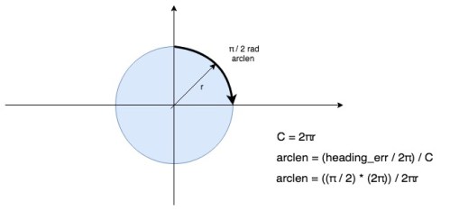
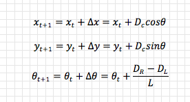
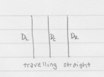
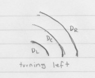
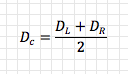
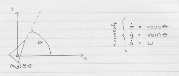
So far, so good. But how can we put this into practice with the wheel(s) of a robot? A common option is to use a rotary encoder such as the Pololu encoder I have used here. This is an optical encoder and uses two infrared reflectance sensors that shine infrared light onto the inside of the wheel hub, upon which is arranged 12 “teeth” with gaps between them.

As the wheel rotates around the shaft of the motor, the teeth pass over the reflectance sensors. When a tooth is above a sensor it reflects infrared light and when no tooth is above it doesn’t. The sensor (after some signal cleaning) outputs a pulse train: high, low, high, low that corresponds to tooth, no tooth, tooth, no tooth. The higher the frequency of the pulse train, the faster the wheel is turning.

A single sensor is good: its pulse train allows us to determine how fast the wheel is rotating, but it lacks a critical bit of information: in which direction is the wheel rotating?

This is where the second sensor comes in. The sensors are physically positioned to provide the same pulse train, but 90 degrees out of phase with one another: a quadrature output signal. When the wheel is rotating in direction A (ie. clockwise) the pulse train from sensor A “leads” that of sensor B (because the tooth passes over A first) and when the wheel is rotating in the opposite direction (ie. counter-clockwise) the pulse train from sensor B “leads” that of sensor A (because the tooth passes over sensor B first).

Screen Shot 2014-10-11 at 2.41.51 PM

Image Courtesy of EDN

Looking at the quadrature output when sensor A leads sensor B (the top two pulse trains, let’s assume this represents clockwise rotation), it can be seen that for a series of consecutive rising and falling edges, the state of the outputs forms the following state table:

Sensor A Sensor B
1 0
1 1
0 1
0 0

Also note that this pattern is cyclical. Once the final state is reached, it will wrap around to the first stage again.

Looking at the quadrature output when sensor B leads sensor A (the lower two pulse trains, let’s assume this is counter-clockwise rotation), it can be seen that for a series of consecutive rising and falling edges, the state of the output forms the following state table:

Sensor A Sensor B
0 1
1 1
1 0
0 0

Notice that the second is exactly the same state table as the first, just “starting” on a different state and transitioning backwards? If so, please collect the big fluffy bear as your prize. The transitions are exactly the same, they just occur in the… opposite direction (because the wheel is rotating in the opposite direction).

Side note: this state table is a gray code, the hamming distance between adjacent states is always 1: only one of the two outputs ever changes its level between adjacent states. If we ever see both outputs change state at the same time then we know there has been an error: there is either noise corrupting the signal or we missed a transition (this latter part is important later on as we’ll be measuring these transitions using interrupts, which, depending on our hardware, could be missed).

To summarise:

  • Our encoder uses an infrared sensor to detect wheel rotation by measuring reflected light bouncing off teeth in the wheel hub
  • The sensor outputs a pulse train that indicates when a tooth is present / not present
  • By counting the pulses we know how many teeth have passed by the sensor
  • By knowing the circumference of the wheel and the number of teeth we can determine the distance the wheel has rotated
  • By measuring the time it took for N teeth to pass, we can determine the velocity of the wheel’s rotation
  • By adding a second sensor, positioned next to the first, we get two identical pulse trains, 90 degrees of out phase with one another
  • Because a tooth must pass over one of the sensors “first”, we can determine the direction of rotation by examining the phasing of the pulse trains

So, if we can get the Beaglebone Black to monitor these pulse trains, we can work out how the wheel is rotating (and as we have two wheels, we’ll end up with two of everything: two encoders, two sets of pulse trains, four individual signals to monitor).

Detecting Interrupts with Beaglebone Black’s GPIOs

As well as the many peripherals (PWMs, ADCs) that can be exposed on the Beaglebone’s external pins, most of them can also act as General Purpose I/Os (GPIOs), capable of acting as inputs (which determine the level of the signal applied to them) or outputs (which generate a signal, ie. to drive an LED or other external device). When configured as inputs they can also generate interrupts on a rising of falling edge of the input signal and this is the functionality that I used to monitor the encoder signals and thus implement the odometer.

Unfortunately, when I was working with the Beaglebone Black it was still quite fiddly to configure the GPIOs. Recall from earlier posts that the BBB has a lot of internal peripherals whose functionality is multiplexed out onto external pins according to the device tree. In order to change what gets mapped onto which pins, device tree overlays are used to reconfigure the hardware at runtime. So I had to write a DTO (Device Tree Overlay) that configured P9_11, P9_13 and P8_7, P8_8 (there is nothing magical about this choice of pins other than that they can act as GPIOs and aren’t being used for the PWM or ADC in this project) as GPIOs in input mode and load this before running my odometer program. Derek Molloy has a great tutorial about using the GPIOs on the BBB and writing / compiling DTOs here. You’ll want to read it if you haven’t before.

Putting this all together, to implement the odometry I had to:

  • Connect the two outputs from each rotary encoder (one per wheel) to external pins on the BeagleBone Black that can act as GPIOs (P9_11, P9_13, P8_7 and P8_8 in my case, these are protected with 100ohm inline resistors)
  • Write and compile a Device Tree Overlay that multiplexes the external pins to GPIOs and configures their hardware as inputs
  • Write some code that uses the virtual files in sysfs to export control of the GPIOs into userland (a directory of virtual control files is created for each GPIO that is exported, Derek’s tutorial discusses this in detail) and then configure the GPIOs as inputs that generate interrupts on both rising and falling edges
  • Write some code that monitors the state of the encoder outputs by waiting for interrupts on the GPIOs and measures the direction and amount of rotation

The code itself is on github and documented, but I wanted to explain in some more detail how the main odometer loop works and the assumptions that it makes. The code performs odometry for two encoders/wheels, but to simplify the explanation below we assume we’re dealing with just one encoder.

  • It tracks five values for each encoder (wheel):
    • The current state (as measured directly after the interrupt, or assumed based on logic) of each sensor (currentA and currentB)
      • Assumed based on logic is… an assumption. If we trust that the phase difference between the two pulse trains is always 90 degrees, that it is only possible for the states to transition between adjacent codes according to the gray code and that we do not miss any interrupts then when an interrupt (rising or falling edge) occurs on one sensor, if we measure the level of that signal we can assume we know the level of the other sensor – because it follows a gray code it cannot have changed since the last interrupt (because only one signal can change a time between adjacent gray code states, and the changing signal must have been the one experiencing the interrupt). This assumption falls apart if we miss an interrupt for any reason (ie. the processor was busy, something got lost in noise etc). In that case, we may not actually be in the state immediately adjacent to the last one we measured: we could be several/hundred/millions of states further on.
    • The previous state (at the last interrupt) of each sensor (lastA and lastB)
    • A counter that increments by one for each forward transition (“tick“) and decrements by one for each backward transition (“tick“) through the state table (odometer).
      • If odometer == 0 and then the wheel rotates forward/clockwise over the course of five consecutive interrupts/ticks, odometer == 5.
      • The Pololu encoder generates 48 ticks per complete revolution of the wheel. Thus, if the wheel has a radius = 2cm and thus a circumference c = 12.57cm, if we see 48 consecutive transitions through the table in a single direction, the wheel has turned 12.57cm. If we see 24 consecutive transitions through the table in one direction, and then 24 consecutive transitions through the table in the opposite direction, the wheel has still turned 12.57cm, but if it were travelling in a straightline over ground it would be back at its origin position.
  • Before looping, it opens 2 file handles, one to each GPIO (we need 2 GPIOs per rotary encoder, one to measure each pulse train)
  • The main loop construct is built around a blocking poll() on the file handles. An interrupt on either of the GPIOs (ie. the detection of a rising or falling edge on one of the encoder output pulse trains) causes the poll to return.
  • It then determines which GPIO had the interrupt and reads the state of that GPIO (ie. the current level of the pulse that just experienced the edge). Going back to the assumptions above, it now “knows” the current level of both sensors: currentA and currentB.
  • It XORs the current level of each sensor against the level of the opposite sensor at the last interrupt (lastA and lastB) which allows it to determine whether it is transitioning “forward” or “backward” through the state table, and thus the direction in which the wheel is rotating. The odometer counter is incremented or decremented accordingly. It also performs a basic sanity check to ensure the current states do not violate the gray code (which probably indicates that we’ve missed an interrupt and cannot be certain of our count any more).

To illustrate, we can walk through several ticks from a reset state and see what happens. To refresh, the gray code for the encoder is:

State Sensor A Sensor B
0 0 0
1 0 1
2 1 1
3 1 0

tick 0 (power on)

Note: This assumes the initial state of the encoder is 0 (ie. sensor A = 0, sensor B = 0). If it’s not we just get an initial gray code violation error, the code could be made more robust by simply measuring the actual starting state).

currentA = 0
currentB = 0
lastA = 0
lastB = 0 
odometer = 0

tick 1 (first interrupt, rising edge on B: state 0 -> state 1)

currentA == 0 (this is assumed, because interrupt occurred on b)
currentB == 1 (this is read now, because interrupt occurred on b)
lastA == 0
lastB == 0

if (currentA ^ lastB) odometer--;   // false
if (currentB ^ lastA) odometer++;   // true

NOTE: The above determines whether the transition is from state 0 to state 1 (forwards) or from state 2 to state 1 (backwards). If lastA 
and lastB had been 1 (ie. previous state was state 2) the odometer would have been decremented.

lastA = currentA = 0
lastB = currentB = 1
odometer == 1

tick 2 (second interrupt, rising edge on A: state1 -> state 2)

currentA == 1 (this is read now, because interrupt occurred on a)
currentB == 1 (this is assumed, because interrupt occurred on a)
lastA == 0
lastB == 1 

if (currentA ^ lastB) odometer--;   // false
if (currentB ^ lastA) odometer++;   // true

lastA = currentA = 1
lastB = currentB = 1
odometer == 2

tick 3 (third interrupt, falling edge on B: state 2 -> state 3)

currentA == 1 (this is assumed, because interrupt occurred on B)
currentB == 0 (this is read now, because interrupt occurred on B)
lastA == 1
lastB == 1

if (currentA ^ lastB) odometer--;   // false
if (currentB ^ lastA) odometer++;   // true

lastA = currentA = 1
lastB = currentB = 0
odometer == 3

tick 4 (fourth interrupt, direction reversed, rising edge on B: state 3 -> state 2)

currentA == 1 (this is assumed, because interrupt occurred on B)
currentB == 1 (this is read now, because interrupt occurred on B)
lastA = 1
lastB = 0

if (currentA ^ lastB) odometer--;   // true
if (currentB ^ lastA) odometer++;   // false

lastA = currentA = 1
lastB = currentB = 1
odometer == 2

Screen Shot 2014-10-11 at 6.33.52 PM

Beaglebone Black Analog to Digital Converter

Goal: Get the robot to drive around the room and avoid obstacles

Once the DRV8833 was hooked up to the two DC micro motors and the BBB’s PWMs, I wrote some simple C++ code to abstract movement (ie. forward(), reverse(), spinLeft(), spinRight() etc). It was now possible to write little programs to move around along a predetermined path. At this point the robot had no idea where it was, but was capable of driving forward for 2 seconds, turning left, doing that some more and making a square for example.

It’s worth noting at this point that although I later took some actual measurements as to the mechanical differences between the two motors and how they each uniquely responded to the same PWM duty cycle, during this early phase a DC of 50% more than adequately drove the robot in a “straight” line for small distances (and it was obvious from trial and error that there was a critical minimum DC at which the motors did not generate enough torque to turn the wheels when in contact with the floor).

Before I delved further into location awareness and odometry, I wanted to test out the Maxbotix MaxSonar-EZ1 ultrasonic transducer that I had bought and get some practice with the BeagleBone’s built-in ADC. The aim was to write a simple finite state machine to:

  1. Drive forward while measuring proximity of objects in front of robot using the ultrasonic transducer
  2. When a “safe” distance threshold was breached, slow down
  3. When a “danger” distance threshold was breached, enact collision avoidance (ie. reverse a bit, spin around, drive forward again)

With the PWMs and DRV8833 all the driving component was taken care of, the major work was in interfacing with the MaxSonar-EZ1.

MaxSonar-EZ1

For hobby work this is one of the kings of ultrasonic sensing (and the price tag reflects it!). In the past I’ve worked with bare 40kHz transducers and built 1573_HRLV-EZ Ultrasonic Range Finder
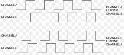
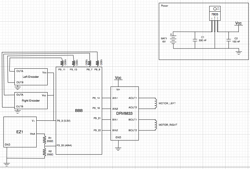
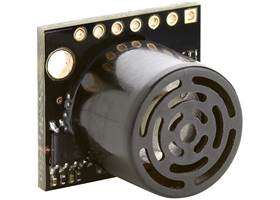
an amplifier and wave generator for them, along with interfacing them back into timers for distance measurement, but a package like the EZ1 takes care of all of this for you.

The EZ1 has a typical 30cm deadzone, but outside of that has excellent resolution (they claim 1mm), a 5m range (I’ve only tested it up to about 3m in my apartment, but it gives linear readings all the way out to that distance) and supports multiple interfaces including analog voltage output (although this decreases the object detection resolution to 5mm), serial over TTL, serial over RS232 and PWM.

I really haven’t explored all the options this thing has to offer because it was so simple to get up and running, but with the other output options and the ability to start and stop its sensing, it can be used a lot more effectively than I’m currently using it here. The datasheet is easy reading and the Quick Start Guide is useful for playing around with it on the bench.

Using the BBB ADC

The MaxSonar-EZ1 supports multiple output methods but for my testing I wanted to use the analog output so I could play around with the BBB’s ADC. The EZ1 can run on anything from 2.5V – 5.5V DC and the analog output voltage it emits to represent distance obviously scales within 0V and the nominated supply voltage. In my case I am powering it from the 3.3V output on the BBB itself (available on pin 3 of the P9 header).

The BBB has a 7 channel ADC with 12-bit resolution. The most important thing to note is that the ADC inputs are 1.8V logic: do not exceed this or you’ll fry it. Because we’re supplying the EZ1 with 3.3V, its analog output (on pin 5 of the EZ1 board) must be put through a voltage divider so the BBB ADC only sees up to 1.8V.

I’m using a simple 50/50 divider built from two 200ohm 0.1% error tolerance resistors, the output of the voltage divider is being fed into pin 33 on P9, which corresponds to AIN4 (the 5th ADC input). It’s important to use low error tolerance resistors because we’re trying to measure a voltage that varies between 0 – 1.8V with a 12-bit resolution (4096 possible values). Technically this gives the ADC the ability to differentiate down to the sub-mV level (ie. one quantisation step represents around 0.44mV: if the resistors skew the real output from the EZ1 then you can lose noticeable accuracy.

The ADC also needs a GND reference connected (pin 34 of the P9 header), I simply connect this to pin 2 of the P9 header which is connected to the BBB ground.

Like with the PWM, on the version of Angstrom that my BBB came with there is a handy module that exposes the readings from the ADC into userland virtual files, called cape-bone-iio. To enable the ADCs the virtual cape itself must first be loaded (as per the PWM the # in the capemgr directory represents a BBB-specific value, your mileage may vary):

# echo cape-bone-iio > /sys/devices/bone_capemgr.#/slots

Each ADC now has its own virtual file that can be read which will return a value between 0 and 1800: the module takes care of converting the 12-bit resolution into an actual mV reading. You’ll see the OCP reference around quite a bit, I believe it stands for “On Chip Peripherals” – all the good stuff that’s baked directly into the AM3359 processor.

# cat /sys/devices/ocp.#/helper.#/AIN4
2049

The MaxSonar-EZ1’s output voltage can be converted into distance using the formula:

Vcc / 512 = mV_per_inch
distance_inches = mv_from_ADC / mv_per_inch

Because I like working in centimeters and the voltage scale the BBB ADC sees is half that of the actual EZ1 Vcc (because of the voltage divider):

distance_cm = (mv_from_ADC * 512 * 2.54) / 1800

Finally, the readings you get from the ADC might bounce around a bit (ie. try putting something solid a fixed distance in front of the uS sensor and then reading the ADC 5 times in a row, once per second). To get around this I sample the ADC several times (32) with a fixed delay between each sample (1ms: the ADC has a sample time of 125nS so this is plenty enough), then I order the samples and select the median. This is a really inefficient way of doing median filtering, there is a paper about much better alternatives here.

Hipster Circuits, the builders of the incredibly cool Replicape 3D printer cape for Beaglebone, note on their BBB ADC post that newer kernels have changed the way that the ADC is accessed and that cape-bone-iio no longer is used.

 Circuit Diagram

Screen Shot 2014-04-01 at 9.16.05 PM