I²C (“Inter-integrated circuit”, which as a trademark of Phillips is more generically implemented by other vendors as “Two Wire Interface” or TWI) is a synchronous serial interface that is often used to connect peripheral devices (think EEPROMs, gyroscopes, accelerometers, wheel encoders etc) to microcontrollers. Electrically, it requires only two “wires” between each device, a clock line (SCL) and a data line (SDA) and these lines can be shared as a common bus between multiple devices, allowing for a multi-master and multi-slave environment. Each slave on the bus has a unique address within a 7-bit address space.

Both the ATmega32U4 (the microcontroller included on the Romi 32U4 control board) and the Raspberry Pi (as functionality included in its Broadcom BCM2835 (or later) SOC), include hardware allowing them to function as either I²C master or slave. This presents an opportunity to allow simple communication between the two. But why would this be useful and how should we choose who gets to be master and who is a slave?

As an 8-bit microcontroller with 32kbyte program memory the ATmega32U4 is clearly limited in its capabilities. There is no room or compute power for more advanced functionality, such as computer vision, that we want oroboto to be capable of. However, if we couple it with a more powerful system, such as the Raspberry Pi, a whole new set of opportunities open up: CV, communication over WiFi, co-operative robotics. The Romi 32U4 control board that the newer iterations of oroboto are using has a female 40-pin header with pinout and mounting holes that are compatible with the Raspberry Pi HAT (Hardware Attached on Top) specification. It directly connects the ATmega32U4’s SDA and SCL lines to those of the Raspberry Pi (which actually has multiple I²C buses) and also routes power from the Romi’s 6x AA batteries to the Pi. You simply have to slot the Pi onto the top of the control board and you now have a powerful robotics platform: the ATmega32U4 can take care of low level functionality like motor control and anything that is timing sensitive, such as reading wheel encoders, and higher level logic, such as navigation strategy and communication can be offloaded to the Pi. Even when adding extra hardware, such as the Raspberry Pi camera, I can power the whole lot for around 45 minutes on the 6x AA batteries.

Having the Raspberry Pi powered up and running alone obviously isn’t sufficient for an integrated system: it needs to be able to communicate with the Arduino via I²C.  However, getting this working can have its complications. There is a known bug in Broadcom Serial Controller (BSC) of the Broadcom BCM2835 SOC (the chip that contains the Raspberry Pi’s CPU, RAM, video and other peripherals such as I²C) that corrupts data when I²C slaves (such as the Arduino) implement a technique known as clock stretching to slow down communication on the bus. It would seem that the hardware TWI (I²C) module in AVR microcontrollers does stretch the clock when the AVR is a slave and this has and is causing trouble for people trying to connect it to a Raspberry Pi because of the Broadcom bug. I should note that I haven’t been able to directly verify whether the Broadcom issue exists in later versions of the BCM283x as used in Raspberry Pi 2 and 3 models.

To work around these issues, the Romi team have created an alternative to the standard Arduino Wire.h I²C library: the PololuRPISlave library which configures the Arduino as an I²C slave and adds timing hacks at the right places to allow successfully communication with a Raspberry Pi master at relatively high speeds. Phew, saved! But… no, oroboto of course has to be more complicated than that.

As previously mentioned, the Romi control board includes the LSM6DS33 IMU (which we need for a gyroscope) and for a while I was also experimenting with a 3-axis magnetometer, the QMC5883L: the readings from both of these units require the Arduino to operate as an I²C master and the sensors as I²C slaves. The pre-canned libraries (which I wasn’t inclined to reimplement) for the LSM6DS33 and QMC5883L configure the Arduino as an I²C master and PololuRPISlave configures it as a slave. Using them together doesn’t work out of the box. While it does seem to be possible to run the Arduino as a mixed master / slave it was a level of fiddling and patching existing libraries I wanted to avoid if possible. The solution I arrived at was counter intuitive from the perspective of “big is master, little is slave” but works: the Arduino remains the single master on the I²C bus and I configure the Raspberry Pi as an I²C slave (even though in the long run it’s the “command module” of the overall integrated system).

The pigpio package (and its Python bindings) expose the bsc_i2c() function that allow the Pi to operate as an I²C slave. After installing pigpio on the Raspberry Pi (it starts a daemon that implements the functionality exposed by its bindings) it’s simple to configure a slave address for the Pi and register for an interrupt when a master attempts to communicate with that address:

import pigpio

pi = None
slave_addr = 0x13

def i2cInterrupt():
   global pi
   global slave_addr
   status, bytes_read, data = pi.bsc_i2c(slave_addr) 

   if bytes_read:
      doYourThing(data)

pi = pigpio.pi()
int_handler = pi.event_callback(pigpio.EVENT_BSC, i2cInterrupt)
pi.bsc_i2c(slave_addr)

Later posts will go into more detail, but the code that runs on oroboto’s Raspberry Pi essentially:

1. Sets up a UDP server listening for data from botLab (the companion macOS application to send commands and receive telemetry from oroboto)
2. Sets up the Raspberry Pi as an I²C slave
3. Is periodically polled by the Arduino (acting as I²C master) to see whether any new commands have arrived from botLab (ie. “navigate to waypoint x,y”)
4. If a command has been received, sends the command payload back to the Arduino for execution

 

 

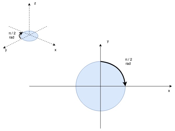
A differential drive robot’s two wheels are placed horizontally adjacent to each other, as if connected by an axle (their “axis”), and their speed is independently controllable. On most (all?) differential drive robots the axis running through the two wheels also runs through the centre of the bot so that any rotation occurs through its centroid in the x-y plane.

As mentioned in the previous post, there are times, such as when a significant correction in heading is required, when we want the robot to “spin on a dime”: that is, rotate around its centroid without changing its (x,y) position. This can be achieved using odometry. In order to rotate π / 2 rad (90 deg) each wheel must travel a distance of arclen, which is defined by the wheelbase (distance between the wheels) of the robot and the desired rotation angle. So, one implementation of rotation can simply be to rotate both wheels in opposite directions at the same speed and periodically (often) check their odometry readings: once they’ve travelled arclen the robot has rotated the required angle.

The problem with this approach is as mentioned in the previous post: the voltage/speed response curves of each motor are not identical. The Romi’s motor libraries accept a signed signed 16-bit integer (capped to -300 to +300) as input, which is converted into a PWM signal to the DRV8838 motor driver, which ultimately is represented as a control voltage to the motor. Instructing both motors to spin at “+100” will result in slightly different actual speeds in each motor. The net result is slip on one wheel (and/or drag on the other) and an invalidation of the assumption that because you’ve measured a distance travelled of d (via odometry) for one wheel that the arclen travelled was really d. In other words, you under or over rotate. While this seems theoretical, in practice it quickly manifests itself. Box test failed.

Luckily, the Romi’s control board has a built-in LSM6DS33 inertial measurement unit. This consists of 3-axis accelerometer and 3-axis gyroscope. Gyroscopes measure rotational motion (angular velocity), that is, how fast they (or the fixed body they’re attached to, in this case, oroboto) are rotating around a given axis. This angular velocity is measured in degrees per second. Just as we can measure (x,y) displacement by integrating translational velocity over time, we can measure angular displacement (rotation) by integrating angular velocity over time.

The course correction mode previously implemented with odometry becomes simpler:

• At t = 0 assume angle_rotated = 0
• Set speed of both motors to s
• Periodically measure (sample) angular velocity around the z-axis (the axis that runs through the center of the robot, “pinning” it to the floor: this corresponds to its change in heading (the interval of this periodic check is dt)
• Integrate the angular velocity with respect to dt, yielding angle_rotated (degrees rotated since t = 0)
• Stop when angle_rotated >= desired rotation

This is a simplification; in the code you can see the LSM6DS33 actually reports angular rotation in “gyrodigits” (digits per second, or DPS), which allow the device to support multiple levels of sensitivity / granularity and that it’s necessary to calibrate the gyroscope before use. Calibration allows some of the random noise the gyroscope experiences to be removed from each sample.

Each sample of the gyroscope’s angular velocity around an axis contains a random amount of noise (ie. some samples will under-report angular velocity, others will over-report angular velocity): continued integration of these samples accumulate that noise and result in drift: the integrated value (ie. the amount of rotation that has occurred since we started measuring) will become less accurate over time. Calibration helps to remove some of this noise but cannot account for all of it. If using the gyroscope to measure rotation over a long time period, this is a problem. Thankfully, course correction routines, where the robot is trying to correct for a specific amount of heading error, are short-lived and essentially “reset the drift clock” each time they start. At the start of the routine, we are seeking to correct for err degrees heading error from the current heading, which for the purposes of the correction, is considered “0 degrees”. The integration of angular velocity only has to occur until err degrees of rotation has occurred from that initial 0 degree starting point. Because this rotation occurs quickly (the robot can spin 360 degrees in under a few seconds, even when moving slowly) there isn’t time for drift to accumulate and as such the gyroscope is accurate under these conditions as illustrated in the videos below.

Drift becomes a problem when trying to use the gyroscope to measure rotational change over a longer time period. Consider a pilot who takes off along a runway with known heading (ie. perhaps it runs due north-south) and who has reset his gyroscope to “0 degrees” when facing north up the runway before takeoff. At this time, the gyroscope reading is accurate. After takeoff, his gyroscope is continually integrating angular velocity (in whichever axes it cares about, hopefully all three) with respect to that initial reset on the runway. Over time, a few hours into his trip, the gyroscope will have accumulated significant error through drift and will no longer be identifying accurate headings. A similar situation occurs with oroboto when using the gyroscope as an alternative to odometry when measuring change in heading between PID loop iterations. In this case the robot continues integrating gyroscope readings as it transits between waypoints, each time adding or subtracting from its last known heading. Over time, gyroscope drift causes these measurements to become less and less accurate and leading to incorrect heading adjustments for the PID loop. Box test failed.

As a method based on integration, odometry suffers exactly the same drift problems as the gyroscope, but in my testing, under the distances travelled (less than 100 meters), odometry was providing better accuracy than the gyroscope method.

One way to correct for drift is to combine the readings of a drift prone sensor (such as a gyroscope or wheel odometry) with the readings of a non-drift prone sensor, such as a magnetometer. This is called sensor fusion, a topic that deserves way more than one post alone.

Before delving into that rabbit hole, however, my next post will focus on interfacing the Romi to a Raspberry Pi I2C slave. This gives oroboto a huge amount of computing power to execute higher level navigational tasks and allows for simple robot-to-robot and robot-to-controller communication over WiFi.

It’s been a long time between posts but I’ve not been idle. I recently discovered the Romi differential-drive chassis from Pololu and have been experimenting with two robots I’ve built on top of it. Unlike the initial iterations of oroboto, which involved a lot of sticky tape and solder bridges to bring everything together on top of the Beaglebone Black (BBB), Romi is a set of neatly interchangeable components including the chassis (with in-built 6xAA battery compartment), 2x 120:1 DC motors, ball caster and wheels. Pololu sell a control board that sits neatly on top of the chassis and provides an ATmega32U4 AVR (Arduino-compatible) microcontroller, DRV8838 H-bridge motor drivers, power distribution circuit and an LSM6DS33 3-axis accelerometer and gyroscope. The motors are easily interfaced with magnetic Hall-effect quadrature encoders to enable odometry and the control board has a header for direct interfacing with a Raspberry Pi. In short, it provides everything the original oroboto had (albeit with a Raspberry Pi rather than a Beaglebone Black) but in a more robust package with less assembly required.

Porting the original oroboto code to the Romi was trivial: all of the interface code that poked the BBB’s GPIOs and interrupts got chucked out and replaced with Arduino-specific library calls but the core PID loop and navigation logic remained. Earlier readers may recall the significant problems I had getting oroboto to “hit its waypoints” while executing a transit. I had hoped the port to Romi would result in immediate performance improvements for two reasons: a) the Romi’s motors were more highly geared (120:1 vs 100:1) which should grant slightly higher rotary encoder resolution, but more importantly; b) everything was running directly on the AVR instead of jumping back and forth between the kernel and user-space on the BBB, which should have resulted in much finer timing and accuracy. The original BBB code relied on a select() on a file descriptor for the user-mode process to learn of GPIO interrupts from the rotary encoder and on a fairly opaque PWM implementation to drive the motors. By the time the feedback loop from input to output was complete there was a lot of context switching and I couldn’t guarantee how the kernel would schedule the oroboto control process. In contrast, on the AVR, everything is running in a single “thread” and timing control is deterministically related only to the running code.

Needless to say, I was disappointed. Well, I wasn’t totally disappointed, it’s always nice after porting a project from one platform to another that it runs at all, but for my “box test” (getting oroboto to transit between 4 waypoints that define the corners of a 1m x 1m square) the accuracy was still fairly miserable. I ruminated on the problem for a few days and realised the obvious: you can’t make pigs fly.

Without giving it due consideration, I think I’d been hoping the PID implementation would magically cause oroboto to spin on a dime once it reached one waypoint and began the transit to the next, but in reality the magnitude of control signal change is often too high to map onto the physical constraints of the motor. Even if it was mappable, such a sudden change in torque can cause slip and inaccurate odometry readings. To be specific, the DC motor speed is varied by controlling its input voltage: this is achieved via a PWM signal sent to the DRV8838 motor driver. Assume the motor’s input voltage range is 0V to 5V and this maps to a (fictitious, I haven’t actually measured min and max RPM)  speed range (post gearing) of 0RPM to 50RPM (discounting for the fact the mapping is not linear, which is a further complication). At any iteration, the PID loop is trying to correct for the heading error (the error between the robot’s current heading and the heading it needs to travel on to reach its target waypoint) by adjusting the speed (RPM) of the left and right motors to create the required amount of “turn” to the left or right. If the robot has reached a waypoint and its next waypoint requires a 90 degree turn to the left (ie. to the adjacent corner of the “box”), the heading error is 90 degrees, which translates into a large positive control signal to right motor (“turn forwards at 200 RPM!”) and a large negative control signal to the left (“turn backwards at 200RPM!”). The main problems in this scenario are that the magnitude of the control signal (as measured in RPM) can exceed the physical capabilities of the motor and that the response curve of each motor (the mapping between input voltage and output RPM) is neither linear nor matched to that of the other motor. While you might hope these differences “come out in the wash”, that wasn’t my experience. The first problem is somewhat akin to the turning circle of a car: you simply can’t turn at an angle greater than that allowed by the physics of the steering mechanism.

I decided to simplify the problem and let the differential-drive robot do what it does best: spin. At each iteration of the PID loop, if the heading error exceeds 30 degrees, I break into a “course correction” mode that stops forward transit and (relatively) slowly spins the motors in opposite directions to achieve the amount of “on a dime” turn required to correct the heading error. Once corrected, I let the PID loop take over “straight line” correction again. This made a significant improvement in accuracy during the box test and even allowed the robot to complete several transits of more complicated box patterns with little displacement error. However, the problem of mismatched response curves between motors remained. During this course correction mode, the arc length that must be travelled by one of the motors to achieve the rotation required to correct for the heading error is computed and then the odometry of that wheel is monitored until the arc length has been traversed: in other words, it assumes that if that wheel has travelled a certain distance then the other wheel has travelled exactly the same distance in the opposite direction and thus that the required rotation has occurred. This is a poor assumption: the motors do not have the same response curves and when instructed to spin at the same speed, a margin of error (which differs based on the requested speed due to non-linearities in the motors themselves) is introduced. The net result is that over or under rotation occurs.

While I did spend some time writing motor calibration code to do simple lookup table based left-to-right response curve correction I settled on a different approach: ditch odometry for the rotation measurement and use the onboard gyroscope instead.

The next few posts will discuss using the LSM6DS33 inertial measurement unit (IMU) gyroscope; why sensor fusion between an accelerometer and gyroscope can’t ever give better measurements of yaw; how to interface the AVR to a Raspberry Pi acting as an I2C slave (and why you might want to do that); introducing peer-to-peer communication over WiFi between two robots for co-operative navigation and using AWS Rekognition and OpenCV to give oroboto eyes.